Warehouse Slotting: Shortening the Pick Path

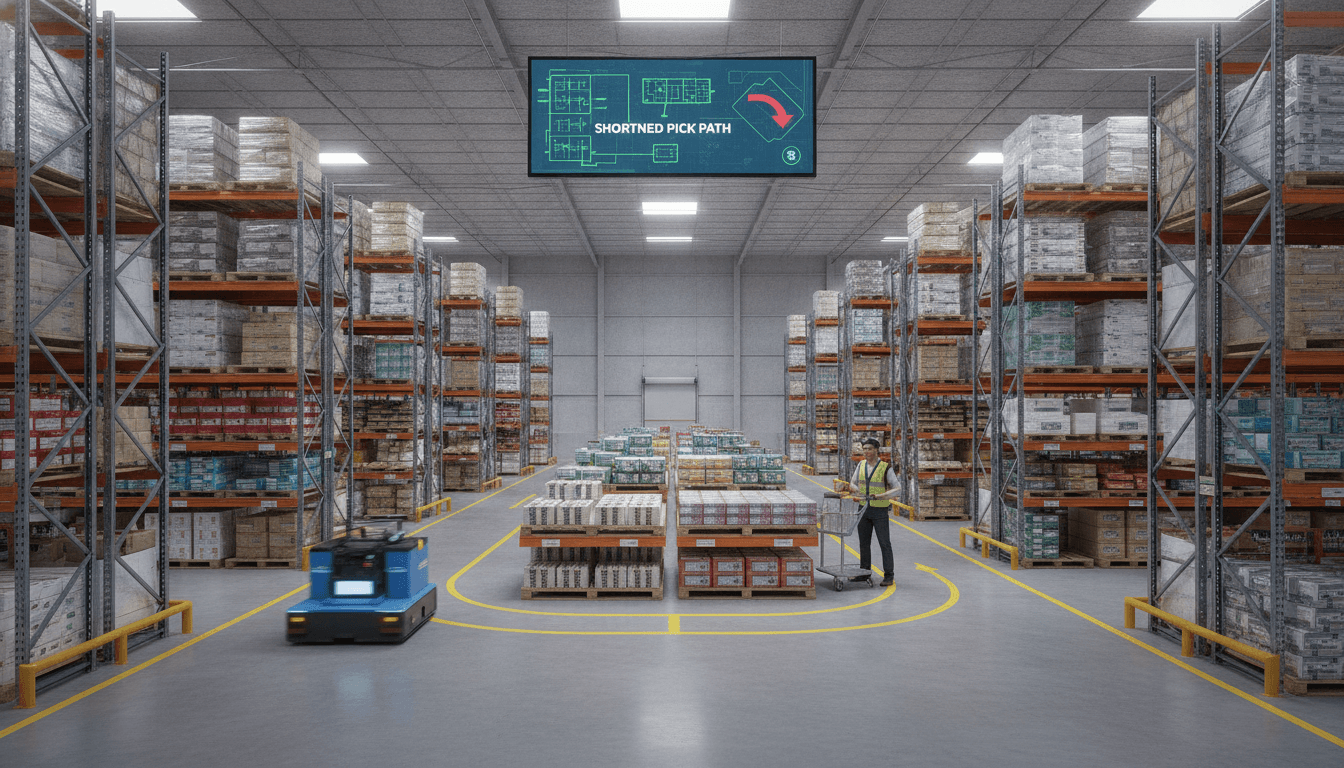
Warehouse slotting decisions made at go-live rarely age well. Six months in, your fastest-moving SKUs are still where you put them during setup, your pick paths have grown by 30%, and your pickers are walking half a kilometre more per order than they need to. Here's a look at how slotting optimisation actually works, what the algorithms are doing, and what it takes to build a system that keeps slot assignments current rather than just correct at launch.

What Is Warehouse Slotting Actually Optimising?

The core problem is a bin-packing variant mixed with a travelling salesman problem. You have a fixed physical space, a set of locations with attributes (height, weight capacity, pick face width, zone, aisle, bay, level), and a catalogue of SKUs with their own attributes (velocity, dimensions, weight, temperature requirements, co-pick affinity). The objective is to assign SKUs to locations such that the total travel distance across all picks in a planning window is minimised, subject to physical and operational constraints.

Travel distance is the primary lever, but it's not the only one. Ergonomic cost matters too. Picks from golden zone locations (roughly 75 cm to 130 cm from the floor) are faster and cause less repetitive strain than floor-level or overhead picks. A good slotting model weights ergonomic cost alongside distance, often by applying a penalty multiplier to out-of-zone picks.

Velocity Classification

Before any slot assignment happens, SKUs get classified by pick frequency. The standard approach is ABC analysis: A items are the top 5–10% of SKUs by pick frequency, accounting for roughly 50–60% of picks. B items are the next 20–30%, accounting for another 30–35%. C items cover the rest.

Some operations extend this to ABCD or even finer buckets. That's usually worth doing when the tail is long and warehouse travel time is a significant cost. For a site picking 10,000 orders a day, shaving 15 seconds per pick across A items compounds quickly.

Co-location and Affinity Clustering

SKUs that appear together in the same order frequently should be slotted close to each other. This is affinity clustering. You build an affinity matrix from historical order data, where each cell represents how often SKU i and SKU j appear in the same order. Then you use clustering algorithms (k-means, hierarchical clustering, or graph partitioning depending on SKU count) to group high-affinity SKUs and assign those groups to adjacent locations.

The challenge is that velocity and affinity can conflict. Two high-affinity SKUs might both be A-class, so they both want to be in the primary pick zone, and that's fine. But if one is A-class and the other is C-class, you need to decide which constraint wins. Typically velocity takes priority, but the model should surface these conflicts explicitly rather than silently resolving them.

How Do You Model the Physical Warehouse?

The warehouse graph is the foundation. Each location is a node. Edges represent traversal routes between locations, weighted by time or distance. For a simple rectangular warehouse with straight aisles, you can compute travel distances analytically. For anything more complex (multiple floors, mezzanines, cross-aisles at irregular intervals, conveyor intersections), you need an explicit graph representation and shortest-path queries.

Most implementations use a simplified rectilinear distance model for speed during optimisation, then validate results against the full graph. The error from rectilinear approximation is usually under 5% for standard warehouse layouts, which is acceptable given other sources of variability in the model.

Zone constraints layer on top of the graph. Refrigerated zones, hazardous materials zones, and high-security zones impose hard constraints that override any optimisation output. Build these as constraint filters that run before the optimisation, not inside it. Mixing hard constraints into the objective function makes the model harder to debug.

What Does the Slotting Algorithm Actually Look Like?

For medium-sized warehouses (up to 20,000 SKUs, up to 50,000 locations), a greedy assignment with local search post-processing is usually fast enough and produces good results. The greedy phase assigns SKUs to locations in velocity order, picking the best available location at each step. Local search then iterates over pairs or triples of assignments and swaps them if the swap reduces total travel cost.

For larger catalogues or more complex constraint sets, you move to metaheuristics. Simulated annealing works well here. You accept worse solutions with a probability that decreases over time, which lets the algorithm escape local optima. A well-tuned simulated annealing run on a 100,000-SKU problem typically converges in 20–40 minutes on a single machine, which is acceptable for a nightly batch job.

Integer linear programming (ILP) with solvers like Gurobi or CPLEX can find provably optimal solutions for smaller problem sizes (under ~5,000 SKUs and locations). Above that, the solve time becomes impractical unless you decompose the problem into sub-problems by zone or product family.

Slot Assignment Output

The output of the optimisation is a slot assignment file: SKU, location, and optionally a recommended put-away date if you're doing a phased slot change. This feeds into your WMS, usually via a bulk import API or a direct database write depending on how the WMS is set up.

One practical note: most warehouse teams can't action a full re-slot of 50,000 locations in one go. Design the output to rank slot changes by expected travel-distance improvement. The top 10% of changes typically deliver 60–70% of the total benefit. Teams can act on those first and defer the rest.

How Often Should You Re-Run Slotting?

Static one-time slotting is almost always wrong. SKU velocity shifts with seasonality, promotions, and product lifecycle. A SKU that's A-class in December might be C-class in March. If your slot assignments don't track that, you're paying a compounding pick-path penalty.

The right cadence depends on how volatile your catalogue is. For a stable catalogue (grocery staples, industrial parts), monthly re-slotting is usually sufficient. For a volatile catalogue (fashion, electronics, seasonal goods), weekly or even daily re-slotting of just the A-class tier makes sense.

Re-slotting has a cost too: labour to move product, disruption during the move, and WMS update time. A sensible model computes the break-even point for each proposed slot change: how many picks at the new location will it take to recover the cost of the move? Only changes that break even within the planning window should be executed.

Re-slot Frequency	Best Fit	Watch Out For
One-time at launch	Stable catalogues, small SKU count	Degrades quickly as demand shifts
Monthly	Most 3PL and distribution centre operations	Misses seasonal spikes
Weekly (A-class only)	Fashion, electronics, promotions	WMS sync overhead
Daily (A-class only)	Very high velocity, short product cycles	Labour cost of frequent moves

What Infrastructure Does a Slotting System Sit On?

The data requirements are straightforward. You need order history (at least 90 days, ideally 12 months for seasonality), SKU master data with physical dimensions, and a location master with physical attributes. If your WMS exports these as flat files or via API, you can pull them into a pipeline built on standard tools: Python with pandas and scipy for the optimisation logic, a PostgreSQL or Redshift instance for the data, and a scheduler (Airflow works fine) for the nightly run.

The heavier investment is integration. Writing slot changes back to the WMS without breaking active picks requires careful transaction management. Most WMS systems have a "freeze" mechanism for locations that are currently being picked; your integration needs to respect that. Test this path thoroughly. A botched slot update mid-shift causes real operational damage.

The slotting engine itself doesn't need to be microservices or cloud-native from day one. A well-written Python script that runs on a scheduled job and produces a ranked change list is genuinely useful. Add infrastructure complexity only when the problem size or the latency requirements actually demand it.

Conclusion

Slotting optimisation is a high-leverage engineering problem that most warehouses either skip entirely or do once and forget. The algorithm choices are well understood; the harder work is data quality, WMS integration, and building a process around regular re-slotting rather than treating it as a project with an end date.

If you're evaluating this for your operation, start with 90 days of order history, run an ABC analysis on your SKU catalogue, and compute your current average pick path length. That baseline will tell you whether slotting is your biggest lever or whether something else (batch optimisation, wave planning) should come first.

FAQ

What's the minimum data needed to run a slotting optimisation? You need order line history (SKU, quantity, timestamp), a location master with aisle, bay, and level coordinates, and SKU dimensions and weight. Ninety days of order history is the practical minimum. Less than that and velocity classifications are unreliable, particularly if your catalogue has any weekly or monthly demand patterns.

Can a WMS like Manhattan, Blue Yonder, or SAP EWM do slotting natively? All three have slotting modules. They're generally adequate for standard ABC velocity-based slotting. Where they fall short is affinity clustering across large catalogues, custom objective functions, and tight integration with demand forecasting. If your needs are standard, the native module is the right starting point. Custom builds make sense when the native tool can't model your constraints.

How long does a warehouse re-slot typically take to execute? That depends entirely on catalogue size and available labour. Moving 1,000 locations typically takes 2–4 hours with a dedicated team. A full re-slot of a 30,000-location DC is usually spread over two to four weeks to avoid disruption. Phased execution, prioritised by expected distance savings, is the standard approach.

Is machine learning needed for slotting, or do classical algorithms work? Classical algorithms (greedy assignment, simulated annealing, ILP) solve the core slotting problem well. Machine learning is useful upstream: demand forecasting to predict future velocity, and anomaly detection to flag SKUs whose velocity is shifting mid-cycle. ML doesn't replace the optimisation layer; it improves the inputs to it.

What's the typical pick-path reduction from a proper re-slot? Studies across distribution centre operations typically show 10–25% reduction in average pick path length after a velocity-and-affinity-based re-slot, compared to a random or launch-time assignment. The higher end of that range tends to apply when the original slotting was done without any optimisation. Results depend heavily on warehouse layout and order profile mix.

Have a project in mind? Contact Sodio Technologies to discuss your requirements and explore the right technology solution for your business.